Write Python

You already build pipelines in code — as a data scientist moving between notebooks and jobs, a backend developer automating a data chore, an analytics engineer maintaining transformation logic — and you're not shopping for a no-code tool. The reasons this API earns a place anyway are practical: connection and I/O boilerplate collapses into one-liners, Polars performance comes with Polars idioms intact, and every pipeline you write is also a diagram a non-developer colleague can open, inspect, and even take over.

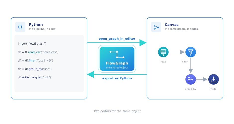
The mental model in one line: every method call adds a node to a graph instead of executing. The graph is the pipeline — Python and the canvas are two editors for the same object.

1. First pipeline

pip install flowfile, then — this snippet is a repository file executed by CI on every commit, so it cannot drift from the real API:

import flowfile as ff

SALES = "https://raw.githubusercontent.com/edwardvaneechoud/flowfile/main/data/templates/supermarket_sales.csv"

revenue_by_line = (
    ff.read_csv(SALES)
    .with_columns((ff.col("unit_price") * ff.col("quantity")).alias("revenue"))
    .filter(ff.col("quantity") > 5)
    .group_by("product_line")
    .agg(ff.col("revenue").sum().alias("total_revenue"))
    .collect()
)

Nothing runs until .collect(): each call appends a node, and collection hands the whole plan to the Polars optimizer at once. The consequences are the useful kind — build a pipeline conditionally, pass it between functions, branch it — all before any data is read. FlowFrame and FlowGraph covers the model, including how branches share one graph and why schemas resolve without executing anything.

2. Your code has a canvas

ff.open_graph_in_editor(result.flow_graph)

That one call is the collaboration story. The pipeline opens in the visual editor as nodes — your colleague walks it step by step, inspects the data between operations, and continues editing visually if that's their medium. Pass description= on operations and those become the node labels, which is what makes a code-built graph legible rather than merely visible. Details in Visual UI Integration.

3. Connectors without ceremony

The boilerplate you're used to writing around sources — credential plumbing, retry-prone connection setup, path handling — is replaced by named connections: create one once (in code or in the UI; both share a single encrypted store) and reference it by name in reads and writes against Postgres/MySQL/SQLite, S3/ADLS/GCS, Kafka, and REST endpoints. The reading and writing references cover every entry point, and the database and cloud examples execute against real services in CI.

4. The catalog from code

The catalog is where scripts and visual flows meet: ff.write_catalog_table publishes a frame as a versioned Delta table anyone can query or chart, and reads come back into any script or notebook. This example round-trips an aggregate through the catalog and back out via SQL — note read_catalog_sql imports from flowfile_frame, one of the API's honest sharp edges:

import flowfile as ff
from flowfile_frame import read_catalog_sql

SALES = "https://raw.githubusercontent.com/edwardvaneechoud/flowfile/main/data/templates/supermarket_sales.csv"

income_by_city = (
    ff.read_csv(SALES)
    .group_by("city")
    .agg(ff.col("gross_income").sum().alias("total_income"))
)

ff.write_catalog_table(
    income_by_city, "docs_sales_by_city", schema=ff.default_schema(), write_mode="overwrite"
)

top_cities = read_catalog_sql(
    "SELECT city, total_income FROM docs_sales_by_city ORDER BY total_income DESC"
)

Catalog References documents the name-based handle API on top of this.

5. Notebooks, next to the data

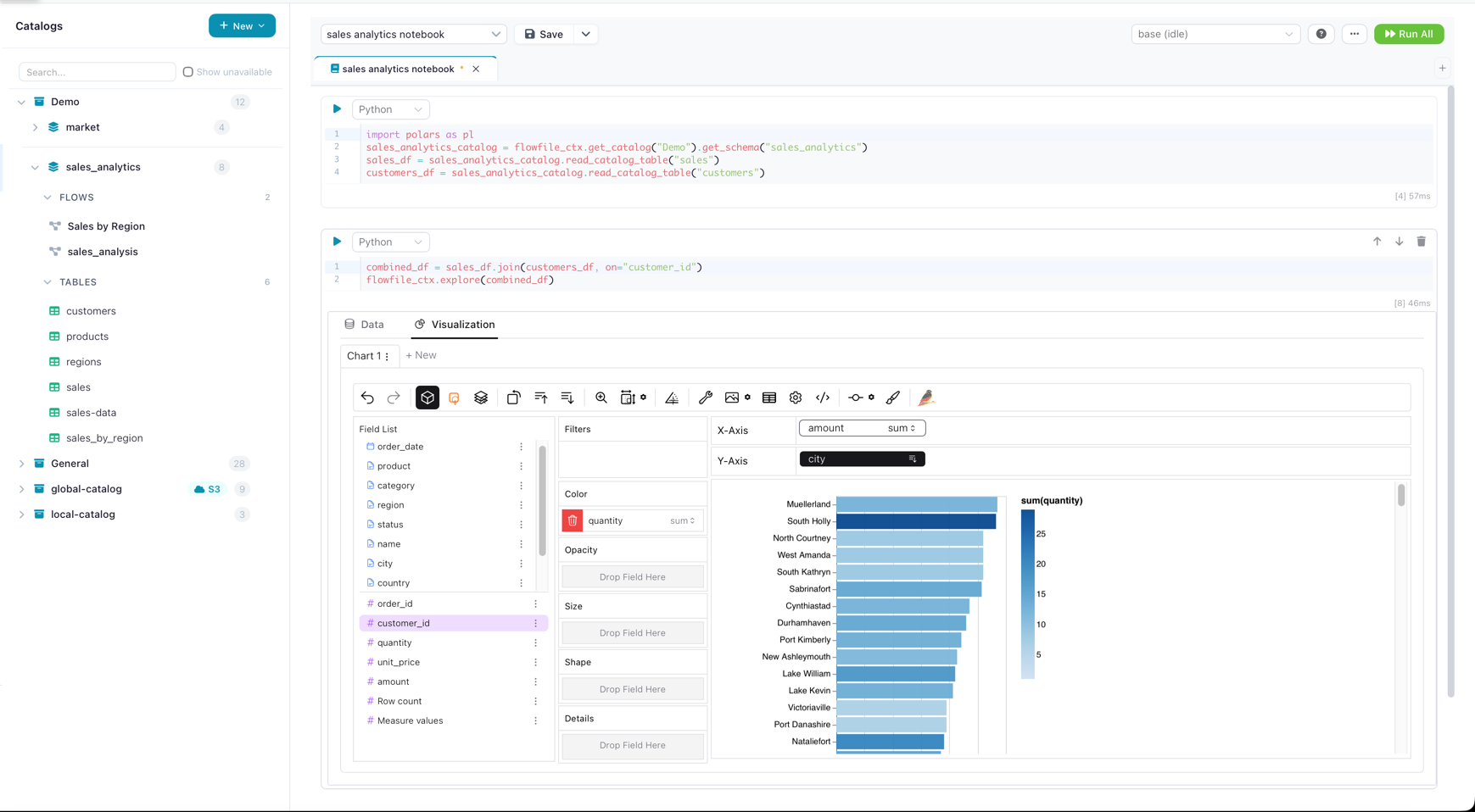
Exploration happens in notebooks — but a local Jupyter detaches from everything: the data gets copied out, the environment drifts from production, and the notebook ends up in a folder nobody else can run. Flowfile's notebooks live in the catalog, next to the tables they analyze, and their Python cells execute on Docker-isolated kernels — any pip library, pinned per kernel, identical for everyone who opens the notebook.

Cells talk to the catalog directly and display like you'd expect — the last expression auto-renders, with richer options a call away:

lf = flowfile_ctx.read_catalog_table("sales_by_city")
flowfile_ctx.explore(lf)   # interactive explorer; .display(lf) for the table view

The editor has code completions, and the same kernel machinery powers the Python Script node when notebook logic graduates into a flow. (Cell code runs inside a kernel — the flowfile_ctx API above is the kernel's, available in notebook cells and the Python Script node but not importable from an ordinary script; a plain script reaches the catalog with the ff.* functions from step 4 instead. Documented in full on The flowfile_ctx API.)

6. Know the two dialects

Two ways to express logic, differing in what the canvas can do with them later:

• Polars-style expressions — ff.col, when/then, the str/dt/list namespaces — feel native and mostly are (Expressions); renames and gaps are listed in the operations reference. Each expression also carries a Flowfile-formula rendering: ff.col("amount") > 100 becomes [amount] > 100, &/| become and/or, and casts plus the str/dt methods map to formula functions. That rendering is why a with_columns built from such expressions lands on the canvas as editable native Formula nodes — the same nodes a canvas user configures by hand. An expression with no formula equivalent becomes a generic code node instead, and filter() given an expression (rather than a formula string) is always a code node.
• Flowfile formula strings — filter(flowfile_formula="[quantity] > 7") — always render as editable native nodes. For filter, the string form is the only one that yields a native Filter node.

Rule of thumb: simple column-derivation steps stay editable on the canvas either way; reach for a code node only when the logic is genuinely code-shaped.

7. Ship and test it

Flows serialize to plain .yaml, which makes the engineering hygiene ordinary: version them in Git, run them headlessly in CI or cron —

flowfile run flow pipeline.yaml --param run_date=2026-07-04

— with exit code 0/1 and no UI or services required. Going the other direction, visual flows export as Python: pure-transformation flows as Polars with no flowfile import (a few formula, fuzzy-match, or graph nodes pull a small polars_* helper), I/O-bearing flows with an ff import for their connections — either way, readable code when a pipeline graduates into a codebase.

---

Fastest first taste: the tested pipeline in step 1 — paste it into any session after pip install flowfile. Then the Python API quickstart for the guided tour, and the reference for the full surface.