Quick Start Guide
Get Started with Flowfile in 5 Minutes
Installation
Recommended quickstart: Install from PyPI
pip install flowfileThis installs everything you need - the Python API, visual editor, and all services.
Want to try Flowfile without installing anything?
Flowfile Lite runs the visual editor entirely in your browser (Polars via WebAssembly) — no install, no signup. Try it at demo.flowfile.org. It's a lightweight subset (18 nodes, no backend, databases, scheduler, or AI); install the full package below for everything else.
Alternative Installation Methods
Desktop Application (Pre-built Installer)
Download the latest installer for your platform: - Windows: Flowfile-Setup.exe - macOS: Flowfile.dmg
Note: You may see security warnings since the installer isn't signed. On Windows, click "More info" → "Run anyway". On macOS, right-click → "Open" → confirm.
Development Setup (From Source)
# Clone repository
git clone https://github.com/edwardvaneechoud/Flowfile.git
cd Flowfile

# Install with Poetry
poetry install

# Start services
poetry run flowfile_worker  # Terminal 1 (port 63579)
poetry run flowfile_core    # Terminal 2 (port 63578)

# Start frontend
cd flowfile_frontend
npm install
npm run dev:web  # Terminal 3 (port 8080)
Choose Your Path
Non-Technical Users
Perfect for: Analysts, business users, Excel power users
No coding required!
- ✅ Drag and drop interface
- ✅ Visual data preview
- ✅ Export to Excel/CSV
- ✅ Built-in transformations
Technical Users
Perfect for: Developers, data scientists, engineers
Full programmatic control!
- ✅ Polars-compatible API
- ✅ Cloud storage integration
- ✅ Version control friendly
- ✅ Complex dynamic logic
Quick Start for Non-Technical Users
Step 1: Start Flowfile, and create a Flow
Open your terminal (Command Prompt on Windows, Terminal on Mac) and type:
flowfile run ui
If the browser does not open automatically
If the browser does not open automatically, you can manually navigate to http://127.0.0.1:63578/ui#/main/designer in your web browser.
Creating your First Flow:
- Click "Create" to create a new data pipeline
- Click "Create New File Here"
- Name your flow (e.g., "Sales Data Analysis")
- Click on "Settings" in the top right to configure your flow
- Set the Execution mode to "Development"
Your should see now an empty flow:
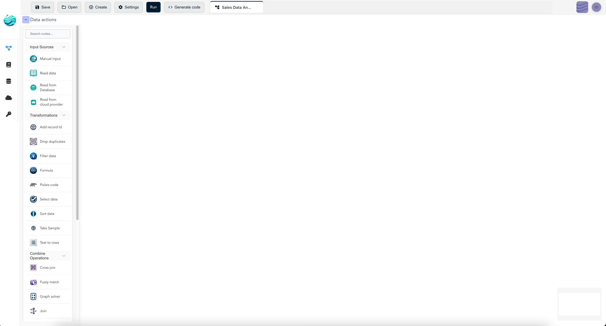 New clean flow interface
Step 2: Load Your Data
Loading a CSV or Excel file:
- Find the "Read Data" node in the left panel under "Input"
- Drag it onto the canvas (center area)
- Click the node to open settings on the right
- Click "Browse" and select your file
- Configure options (if needed):
- For CSV: Check "Has Headers" if your file has column names
- For Excel: Select the sheet name
- Click "Run" (top toolbar) to load the data
- Click the node to preview your data in the bottom panel
Step 3: Clean Your Data
Let's remove duplicate records and filter for high-value transactions:
Remove Duplicates
- Drag "Drop Duplicates" node from Transform section
- Connect it to your Read Data node
- Select columns to check for duplicates
- Click Run
Filter Data
- Drag "Filter Data" node from Transform section
- Connect it to Drop Duplicates node
- Enter formula:
[Quantity] > 7 - Click Run
Step 4: Analyze Your Data
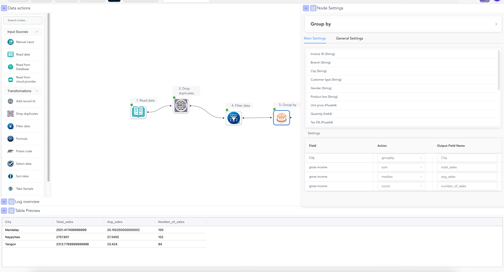
Create a summary by city:
- Add a Group By node from the Aggregate section
- Connect it to your Filter node
- Configure the aggregation:
- Group by:
city - Aggregations:
gross income→ Sum → Name ittotal_salesgross income→ Average → Name itavg_salegross income→ Count → Name itnumber_of_sales
- Click Run to see your summary
Data after group by
Step 5: Save Your Results
Export your cleaned data:
- Add a "Write Data" node from Output section
- Connect it to your final transformation
- Choose format:
- Excel: Best for sharing with colleagues
- CSV: Best for Excel/Google Sheets
- Parquet: Best for large datasets
- Set file path (e.g.,
cleaned_sales.xlsx) - Click Run to save
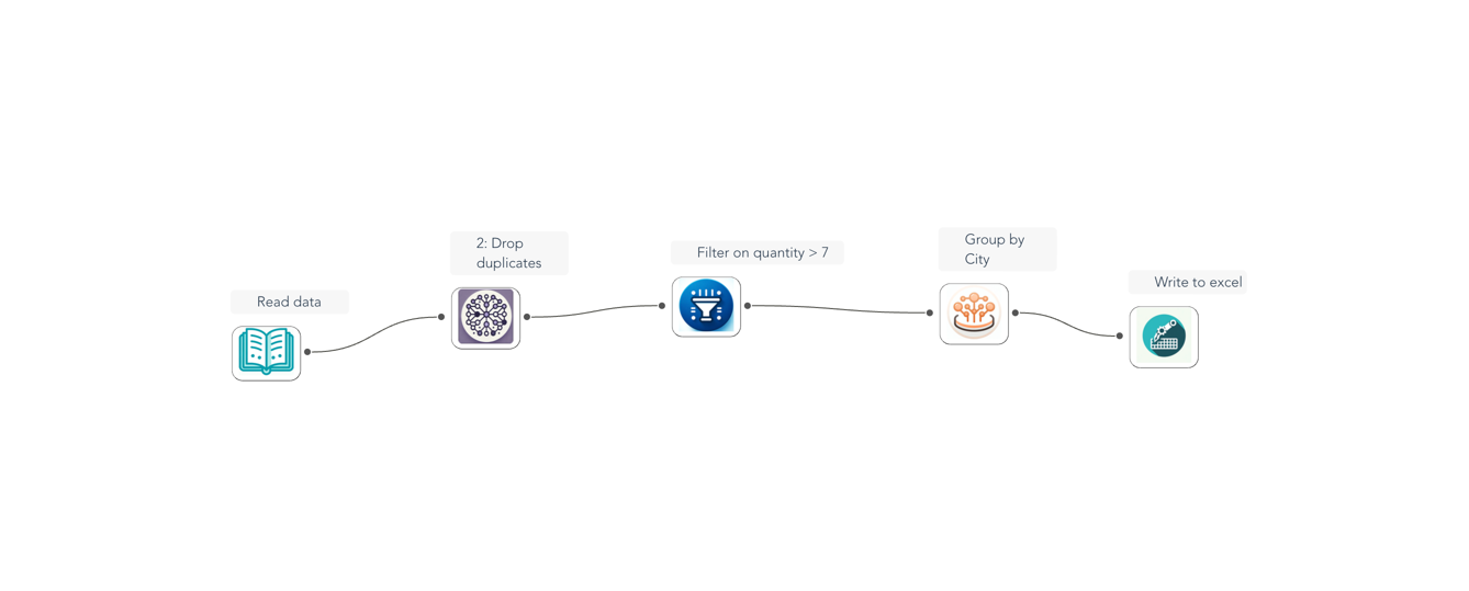
Here's what your complete flow should look like:
Congratulations!
You've just built your first data pipeline! You can:
- Save this flow using File → Save (creates a .flowfile)
- Share it with colleagues who can run it without any setup
- Schedule it to run automatically (coming soon)
- Export as Python code if you want to see what's happening behind the scenes
Pro Tips for Non-Technical Users:
- Use descriptions: Right-click nodes and add descriptions to document your work
- Preview often: Click nodes after running to see data at each step
- Start small: Test with a sample of your data first
- Save versions: Save different versions of your flow as you build
Next Steps
Quick Start for Technical Users
Step 1: Install and Import
pip install flowfile
import flowfile as ff
from flowfile import col, when, lit
import polars as pl  # Flowfile returns Polars DataFrames
Step 2: Build a Real-World ETL Pipeline
Let's build a production pipeline that reads from S3, transforms data, and writes results:
# Configure S3 connection (one-time setup)
from pydantic import SecretStr

import flowfile as ff

ff.create_cloud_storage_connection_if_not_exists(
    ff.FullCloudStorageConnection(
        connection_name="production-data",
        storage_type="s3",
        auth_method="access_key",
        aws_region="us-east-1",
        aws_access_key_id="AKIAIOSFODNN7EXAMPLE",
        aws_secret_access_key=SecretStr("wJalrXUtnFEMI/K7MDENG")
    )
)
Step 3: Extract and Transform
# Build the pipeline (lazy evaluation - no data loaded yet!)
import flowfile as ff
pipeline = (
    # Extract: Read partitioned parquet files from S3
    ff.scan_parquet_from_cloud_storage(
        "s3://data-lake/sales/year=2024/month=*",
        connection_name="production-data",
        description="Load Q1-Q4 2024 sales data"
    )

    # Transform: Clean and enrich
    .filter(
        (ff.col("status") == "completed") &
        (ff.col("amount") > 0),
        description="Keep only valid completed transactions"
    )

    # Add calculated fields
    .with_columns([
        # Business logic
        (ff.col("amount") * ff.col("quantity")).alias("line_total"),
        (ff.col("amount") * ff.col("quantity") * 0.1).alias("tax"),

        # Date features for analytics
        ff.col("order_date").dt.quarter().alias("quarter"),
        ff.col("order_date").dt.day_of_week().alias("day_of_week"),

        # Customer segmentation
        ff.when(ff.col("customer_lifetime_value") > 10000)
            .then(ff.lit("VIP"))
            .when(ff.col("customer_lifetime_value") > 1000)
            .then(ff.lit("Regular"))
            .otherwise(ff.lit("New"))
            .alias("customer_segment"),

        # Region mapping
        ff.when(ff.col("state").is_in(["CA", "OR", "WA"]))
            .then(ff.lit("West"))
            .when(ff.col("state").is_in(["NY", "NJ", "PA"]))
            .then(ff.lit("Northeast"))
            .when(ff.col("state").is_in(["TX", "FL", "GA"]))
            .then(ff.lit("South"))
            .otherwise(ff.lit("Midwest"))
            .alias("region")
    ], description="Add business metrics and segments")

    # Complex aggregation
    .group_by(["region", "quarter", "customer_segment"])
    .agg([
        # Revenue metrics
        ff.col("line_total").sum().alias("total_revenue"),
        ff.col("tax").sum().alias("total_tax"),

        # Order metrics
        ff.col("order_id").n_unique().alias("unique_orders"),
        ff.col("customer_id").n_unique().alias("unique_customers"),

        # Performance metrics
        ff.col("line_total").mean().round(2).alias("avg_order_value"),
        ff.col("quantity").sum().alias("units_sold"),

        # Statistical metrics
        ff.col("line_total").std().round(2).alias("revenue_std"),
        ff.col("line_total").quantile(0.5).alias("median_order_value")
    ])

    # Final cleanup
    .sort(["region", "quarter", "total_revenue"], descending=[False, False, True])
    .filter(ff.col("total_revenue") > 1000)  # Remove noise
)

# Check the execution plan (no data processed yet!)
print(pipeline.explain())  # Shows optimized Polars query plan
Step 4: Load and Monitor
# Option 1: Write to cloud storage
pipeline.write_parquet_to_cloud_storage(
    "s3://data-warehouse/aggregated/sales_summary_2024.parquet",
    connection_name="production-data",
    compression="snappy",
    description="Save aggregated results for BI tools"
)

# Option 2: Write to Delta Lake for versioning
pipeline.write_delta(
    "s3://data-warehouse/delta/sales_summary",
    connection_name="production-data",
    write_mode="append",  # or "overwrite"
    description="Append to Delta table"
)

# Option 3: Collect for analysis
df_result = pipeline.collect()  # NOW it executes everything!
print(f"Processed {len(df_result):,} aggregated records")
print(df_result.head())
Step 5: Advanced Features
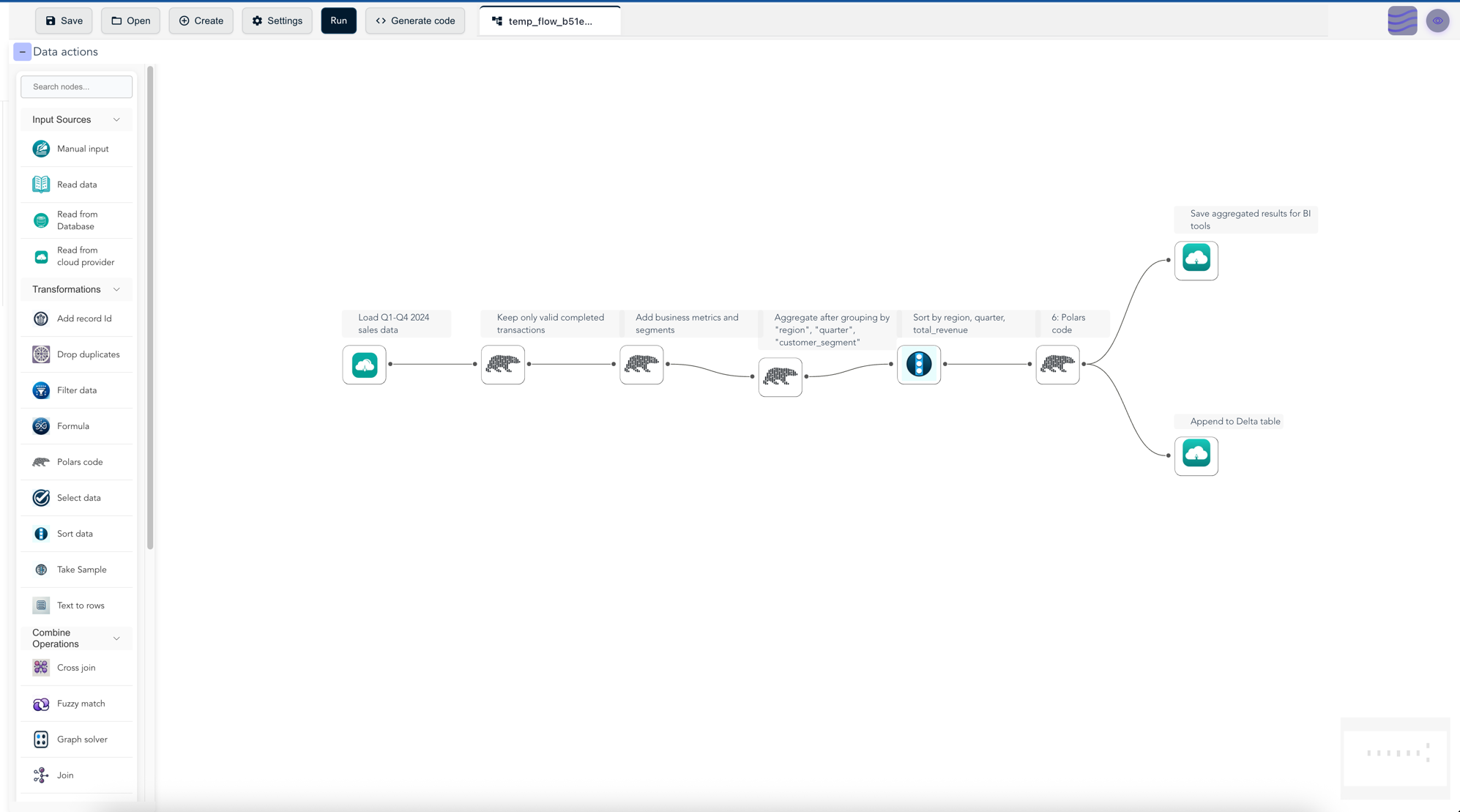
Visualize Your Pipeline
# Open in visual editor
ff.open_graph_in_editor(pipeline.flow_graph)

# This shows your entire pipeline
# as a visual flow diagram!
Visual overview of pipeline
Export as Pure Python
# Generate standalone code
code = pipeline.flow_graph.generate_code()

# Deploy without Flowfile dependency!
# Uses only Polars
Step 6: Production Patterns
Pattern 1: Data Quality Checks
from datetime import datetime
import flowfile as ff

def data_quality_pipeline(df: ff.FlowFrame) -> ff.FlowFrame:
    """Reusable data quality check pipeline"""

    # Record initial count
    initial_count = df.select(ff.col("*").count().alias("count"))

    # Apply quality filters
    clean_df = (
        df
        # Remove nulls in critical fields
        .drop_nulls(subset=["order_id", "customer_id", "amount"])

        # Validate data ranges
        .filter(
            (ff.col("amount").is_between(0, 1000000)) &
            (ff.col("quantity") > 0) &
            (ff.col("order_date") <= datetime.now())
        )

        # Remove duplicates
        .unique(subset=["order_id"], keep="first")
    )

    # Log quality metrics
    final_count = clean_df.select(ff.col("*").count().alias("count"))
    print(f"Initial count: {initial_count.collect()[0]['count']}")
    print(f"Final count after quality checks: {final_count.collect()[0]['count']}")
    return clean_df
Pattern 2: Incremental Processing
# Read only new data since last run
from datetime import datetime
import flowfile as ff
last_processed = datetime(2024, 10, 1)

incremental_pipeline = (
    ff.scan_parquet_from_cloud_storage(
        "s3://data-lake/events/",
        connection_name="production-data"
    )
    .filter(ff.col("event_timestamp") > last_processed)
    .group_by(ff.col("event_timestamp").dt.date().alias("date"))
    .agg([
        ff.col("event_id").count().alias("event_count"),
        ff.col("user_id").n_unique().alias("unique_users")
    ])
)

# Process and append to existing data
incremental_pipeline.write_delta(
    "s3://data-warehouse/delta/daily_metrics",
    connection_name="production-data",
    write_mode="append"
)
Pattern 3: Multi-Source Join
# Combine data from multiple sources
import flowfile as ff

customers = ff.scan_parquet_from_cloud_storage(
    "s3://data-lake/customers/",
    connection_name="production-data"
)

orders = ff.scan_csv_from_cloud_storage(
    "s3://raw-data/orders/",
    connection_name="production-data",
    delimiter="|",
    has_header=True
)

products = ff.read_parquet("local_products.parquet")

# Complex multi-join pipeline
enriched_orders = (
    orders
    .join(customers, on="customer_id", how="left")
    .join(products, on="product_id", how="left")
    .with_columns([
        # Handle missing values from left joins
        ff.col("customer_segment").fill_null("Unknown"),
        ff.col("product_category").fill_null("Other"),

        # Calculate metrics
        (ff.col("unit_price") * ff.col("quantity") *
         (ff.lit(1) - ff.col("discount_rate").fill_null(0))).alias("net_revenue")
    ])
)

# Materialize results
results = enriched_orders.collect()
Next Steps for Technical Users
🌟 Why Flowfile?
⚡ Performance
Built on Polars - Uses the speed of Polars
🔄 Dual Interface
Same pipeline works in both visual and code. Switch anytime, no lock-in.
📦 Export to Production
Generate pure Python/Polars code. Deploy anywhere without Flowfile.
☁️ Cloud Support
Direct S3/cloud storage support, no need for expensive clusters to analyse your data
Troubleshooting
Installation Issues
# If pip install fails, try:
pip install --upgrade pip
pip install flowfile

# For M1/M2 Macs:
pip install flowfile --no-binary :all:

# Behind corporate proxy:
pip install --proxy http://proxy.company.com:8080 flowfile
Port Already in Use
# Find what's using port 63578
lsof -i :63578  # Mac/Linux
netstat -ano | findstr :63578  # Windows

# Kill the process or use different port:
FLOWFILE_PORT=8080 flowfile run ui
Get Help
Ready to Transform Your Data?
Join thousands of users building data pipelines with Flowfile