Technical Architecture

Flowfile's architecture pairs visual design with data processing across three services, built on Polars' lazy evaluation. This page explains the three-service architecture, key technical features such as real-time schema prediction and efficient data exchange, and the role of Polars' lazy evaluation.

Process & execution map

Flowfile runs as several cooperating processes. The Frontend talks only to Core; Core orchestrates everything else and never materializes full datasets itself — heavy compute is offloaded. The diagram shows every process and how the five kinds of execution flow through them.

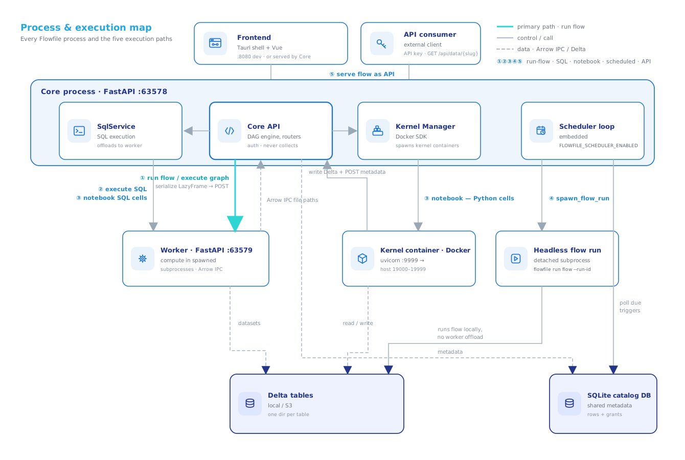
The five execution paths:

Run flow / execute graph — Core builds the LazyFrames, serializes them, and POSTs to the Worker, which holds dataset memory in spawned subprocesses and returns Arrow-IPC paths. Core ships paths, never collected frames.
Execute SQL (SQL editor and catalog SQL) — Core's SqlService registers the catalog tables and runs the query on the Worker.
Execute a notebook — Python cells run in the bound kernel container (which writes results to Delta and POSTs metadata back to Core); SQL cells take path ②; Markdown renders client-side.
Scheduled run — the embedded scheduler loop (only when FLOWFILE_SCHEDULER_ENABLED) polls the catalog DB for due triggers and launches a detached headless subprocess that runs the flow locally.
Serve a flow as an API — a registered flow is published under /flow-api (JWT-managed); the public, API-key-authenticated GET /api/data/{slug} then runs it synchronously and returns the output of its single api_response node as JSON. One key can call several published flows (routes/flow_api.py, routes/api_consumers.py).

The scheduler is not a separate service — it's a loop inside the Core process. The separate OS processes are the Frontend, Core, Worker (plus its compute children), the kernel containers, and each spawned headless run.

Core Components

Three-Service Architecture

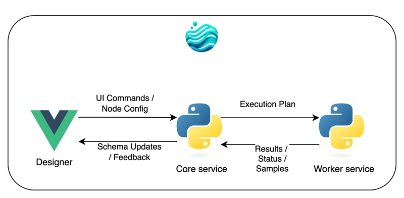
Simplified three-service view: Designer, Core, and Worker. Kernels and the scheduler were added later — see the process map above.

Designer (Tauri + Vue) The visual interface where data pipelines are built through drag-and-drop operations. It is a Tauri 2 desktop shell (Rust) wrapping a Vue 3 renderer, and the same renderer serves the web build. It communicates with the Core service for real-time feedback and data previews.

Core Service (FastAPI) The orchestration engine that manages workflows, predicts schemas, and coordinates execution. It maintains the Directed Acyclic Graph (DAG) structure and handles all UI interactions and overall flow logic.

Worker Service (FastAPI) Handles heavy data computations in isolated processes. It executes Polars transformations, materializes data, and manages data caching using Apache Arrow IPC format, preventing large datasets from overwhelming the Core service.

Key Technical Features

Real-time Schema Prediction

When you add or configure a node, Flowfile immediately shows how your data structure will change — without executing any transformations. This happens through:

Schema Callbacks: Custom functions, defined per node type, that calculate output schemas based on node settings and input schemas.
Lazy Evaluation: Leveraging Polars' ability to determine the schema of a planned transformation (LazyFrame) without processing the full dataset.

View Schema Prediction Python Example

# Example: Schema prediction for a Group By operation
def schema_callback():
    output_columns = [(c.old_name, c.new_name, c.output_type) for c in group_by_settings.groupby_input.agg_cols]
    depends_on = node.node_inputs.main_inputs[0]
    input_schema_dict: Dict[str, str] = {s.name: s.data_type for s in depends_on.schema}
    output_schema = []
    for old_name, new_name, data_type in output_columns:
        data_type = input_schema_dict[old_name] if data_type is None else data_type
        output_schema.append(FlowfileColumn.from_input(data_type=data_type, column_name=new_name))
    return output_schema

The Directed Acyclic Graph (DAG): The Foundation of Workflows

As you add and connect nodes, Flowfile builds a Directed Acyclic Graph (DAG) where:

Nodes represent data operations (read file, filter, join, write to database, etc.).
Edges represent the flow of data between operations.

The DAG is managed by the FlowGraph class (flowfile_core/flowfile_core/flowfile/flow_graph.py) in the Core service, which orchestrates the entire workflow. The class shape below is illustrative — see the Python API Reference for the real signatures.

View FlowGraph shape (illustrative)

class FlowGraph:
    """
    Manages the ETL workflow as a DAG. Stores nodes, dependencies,
    and settings, and handles the execution order.
    """
    uuid: str
    _node_db: Dict[Union[str, int], FlowNode]  # Internal storage for all nodes
    _flow_starts: List[FlowNode]               # Nodes that initiate data flow (e.g., readers)
    _node_ids: List[Union[str, int]]           # Tracking node identifiers
    flow_settings: schemas.FlowSettings        # Global configuration for the flow

    def add_node_step(self, node_id: Union[int, str], function: Callable,
                      node_type: str, **kwargs) -> None:
        """Adds a new FlowNode to the graph."""
        ...

    def run_graph(self) -> RunInformation:
        """Executes the flow in the correct topological order."""
        ...

Each FlowNode in the graph encapsulates its dependencies, transformation logic, and output schema. This lets Flowfile determine execution order, track data lineage, optimize performance, and predict schemas throughout the pipeline.

Execution Modes

Canonical explanation

This is the reference description of Development vs Performance mode. The Core Developer Guide and Design Philosophy pages link here rather than repeat it.

By clicking on settings → execution modes you can set how the flow will be executed the next time you run the flow.

execution settings

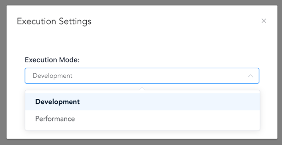
Flowfile offers two execution modes tailored for different needs:

Feature	Development Mode	Performance Mode
Purpose	Interactive debugging, step inspection	Optimized execution for production/speed
Execution	Executes node-by-node	Builds full plan, executes minimally
Data Caching	Caches intermediate results per step	Minimal caching (only if specified/needed)
Preview Data	Available for all nodes	Only for final/cached nodes
Memory Usage	Potentially higher	Generally lower
Speed	Moderate	Faster for complex flows

Development Mode In Development mode, each node's transformation is triggered sequentially within the Worker service. Its intermediate result is typically serialized using Apache Arrow IPC format and cached to disk. This allows you to inspect the data at each step in the Designer via small samples fetched from the cache.

Performance Mode In Performance mode, Flowfile fully embraces Polars' lazy evaluation. The Core service constructs the entire Polars execution plan based on the DAG. This plan (LazyFrame) is passed to the Worker service. The Worker only materializes (executes .collect() or .sink_*()) the plan when an output node (like writing to a file) requires the final result, or if a node is explicitly configured to cache its results (node.cache_results). This minimizes computation and memory usage by avoiding unnecessary intermediate materializations.

View Performance Mode Python Example (simplified)

# Execution logic in Performance Mode (simplified)
def execute_performance_mode(self, node: FlowNode, is_output_node: bool):
    """Handles execution in performance mode, leveraging lazy evaluation."""
    if is_output_node or node.cache_results:
        # If the result is needed (output or caching), offload to the Worker.
        # Offload happens inside ExternalDfFetcher.__init__ — constructing it
        # serializes the LazyFrame and POSTs it to the worker. flow_id and
        # node_id are required.
        fetcher = ExternalDfFetcher(
            flow_id=node.flow_id,
            node_id=node.node_id,
            lf=node.get_resulting_data().data_frame,  # the LazyFrame plan
            file_ref=node.hash,                        # unique reference for caching
            wait_on_completion=False,                  # usually async
        )
        result = fetcher.get_result()  # Worker runs .collect()/.sink_*() and caches
        return result
    else:
        # Intermediate nodes just pass the LazyFrame plan along — no compute here.
        return node.get_resulting_data().data_frame

Crucially, all actual data processing and materialization of Polars DataFrames/LazyFrames happens in the Worker service. This separation prevents large datasets from overwhelming the Core service, ensuring the UI remains responsive.

Efficient Data Exchange

Flowfile uses Apache Arrow IPC format for efficient inter-process communication between the Core and Worker services:

Worker Processing & Serialization: When the Worker needs to materialize data (either for intermediate caching in Development mode or final results), it computes the Polars DataFrame. The resulting DataFrame is serialized into the efficient Arrow IPC binary format.
Disk Caching: This serialized data is saved to a temporary file on disk. This file acts as a cache, identified by a unique hash (file_ref). The Worker informs the Core that the result is ready at this file_ref.
Core Fetching: If the Core (or subsequently, another Worker task) needs this data, it uses the file_ref to access the cached Arrow file directly. This avoids sending large datasets over network sockets between processes.
UI Sampling: For UI previews, the Core requests a small sample (e.g., the first 100 rows) from the Worker. The Worker reads just the sample from the Arrow IPC file and sends only that lightweight data back to the Core, which forwards it to the Designer.

This ensures responsiveness, memory isolation, and efficiency.

Here is how the Core offloads computation to the Worker, and how the Worker manages the separate process execution:

View Core-Side Python Example (simplified)

# Core side - Initiating remote execution in the Worker (simplified)
def execute_remote(self, performance_mode: bool = False) -> None:
    """Offloads the execution of a node's LazyFrame to the Worker service."""
    # Constructing ExternalDfFetcher IS the offload: __init__ serializes the
    # LazyFrame and sends it to the worker (no separate "start" call). The
    # constructor requires flow_id and node_id.
    fetcher = ExternalDfFetcher(
        flow_id=self.flow_id,
        node_id=self.node_id,
        lf=self.get_resulting_data().data_frame,  # the Polars LazyFrame plan
        file_ref=self.hash,                        # unique identifier for result/cache
        wait_on_completion=False,                  # operate asynchronously
    )

    # Store the fetcher to retrieve results later
    self._fetch_cached_df = fetcher

    # For UI updates, request a sample separately
    self.store_example_data_generator(fetcher)  # fetches sample async

View Worker-Side Python Example (simplified)

# Worker side - Managing computation in a separate process (simplified)
def start_process(
    polars_serializable_object: bytes, # Serialized LazyFrame plan
    task_id: str,
    file_ref: str, # Path for cached output (Arrow IPC file)
    # ... other args like operation type
) -> None:
    """Launches a separate OS process to handle the heavy computation."""
    # The worker forces spawn at module load (set_start_method('spawn',
    # force=True) in flowfile_worker/__init__.py) so every child is a fresh,
    # killable process regardless of platform — never fork.
    mp_context = get_context('spawn')

    # Shared memory/queue for progress tracking and results/errors
    progress = mp_context.Value('i', 0) # Shared integer for progress %
    error_message = mp_context.Array('c', 1024) # Shared buffer for error messages
    queue = mp_context.Queue(maxsize=1) # For potentially passing back results (or file ref)

    # Define the target function and arguments for the new process
    process = mp_context.Process(
        target=process_task, # The function that runs Polars .collect()/.sink()
        kwargs={
            'polars_serializable_object': polars_serializable_object,
            'progress': progress,
            'error_message': error_message,
            'queue': queue,
            'file_path': file_ref, # Where to save the Arrow IPC output
            # ... other necessary kwargs
        }
    )
    process.start() # Launch the independent process

    # Monitor the task (e.g., update status in a database, check progress)
    handle_task(task_id, process, progress, error_message, queue)

Lazy Evaluation

By building on Polars' lazy evaluation, Flowfile achieves:

Memory Efficiency: Data is loaded and processed only when necessary, often streaming through operations without loading entire datasets into memory at once. This allows processing datasets larger than RAM.
Query Optimization: Polars analyzes the entire execution plan and can reorder, combine, or eliminate operations for maximum efficiency.
Parallel Execution: Polars automatically parallelizes operations across all available CPU cores during execution.
Predicate Pushdown: Filters and selections are applied as early as possible in the plan, often directly at the data source level (like during file reading), minimizing the amount of data that needs to be processed downstream.

Background reading: the original design article covers the motivation and early design. It predates some renames (the graph class is now FlowGraph, nodes are FlowNode), so treat class names there as historical.